2010-01-15

Astrometry Calibration

I added experimental support for astrometry to Munipack. It is primary designed for astrometry on CCD. So only gnomonical projection and affine transformation (shift and rotation) are supported yet. Both limitation can be freed in future releases.

The astrometry code is available in GoogleCode now.

The algorithm

I coded my own implementation of the widely-known "Astrography plate
measurement" (Smart & Green, Tagg).

On input:
The table with Right Ascension,Declination (from any catalogue) and corresponding measured rectangular x and y coordinates for every object.

The algorithm:
  1. Get center of a picture in pixels as half of both sizes.
  2. Estimate a center of projection in spherical coordinates by mean.
  3. Project spherical coordinates to rectangular ones.
  4. Estimate scale as mean ratio between distances of projected and measured distances of objects.
  5. Estimate angle of rotation between projected and measured coordinates by using of property of scalar product of vectors.
  6. Compute the transformation by some minimization method with starting values given by items 3,4 and 5.
  7. Check offsets between center of projected and measured coordinates. If one is too great, does better estimate of the center of projection and repeat from item 2, else finish.
On output:
Precise coordinates of center of projection, scale and position angle of image. Optionally, statistical parameters.

The described algorithm is relative general, so it can be easy modifies for another projections or more complex transformations of rectangular coordinates like distortions, pincushion, etc.

The algorithm is iterative due to fact that we need known the center of projection before we have calibrated image. Usually, only tree iterations are required.

The Robust Algorithm

The real-world usable algorithm needs to be robust. Small deviations can cause only small variances in output parameters. Outliners has only small fluency on the solution. The simple example of the use of robust method can be found in Launer & Wilkinson: Robustness in statistics: proceedings of a workshop (1979) or in Numerical Recipes. Munipack implements robust mean estimator in lib/statistics.f90 as rmean. Another use of the robust algorithm is on straight light fitting.

I applied the basic schema of robust algorithms to the above algorithm:
  1. Estimate median of absolute deviations (MAD) using of minimization of absolute deviation (Nelder-Mead).
  2. Use method of maximal likelihood to estimate the proper transformation.
Astrometry implements module in astrometry/astrometry.f90. The estimation of MAD is loop around nelmin. The maximum likelihood is loop around Minpack's hybrd.

The fitting is decomposed on tree single steps (estimate of center of projection, scale and affine transformation) so we works in parameter sub-spaces (we are not fitting all the parameters together). Numerical experiments gives me more robust behavior and more precise solutions than simultaneous fitting of all parameters. By my opinion, it is results of (non-)ignoring of their cross-correlations. It is interesting that QR decomposition does not solve the problem.

The algorithm is optimized on precision not on speed. So for a lot of objects may be slow.

The Low Precision Algorithm

The robust algorithm can be used only for many object (ideally for tens of stars and more). The absolute minimum is five stars. I'm supposing that sometimes will be required astrometry for less stars. In this case, I'm switching to a simple algorithm which uses median only to estimate of required parameters.

For two stars, the transformation can be determined, but is is not possible to estimate uncertainties of parameters. It is not possible to estimate scale or rotation for only single star.

Input/Output "protocols"

I choose an unusual way to set an input and get an output data. The stream input is a text file consists a set of lines (records) with the same structure as FITS headers. By the user point of view, the routine performs as a transformation filter. The text file on input is modified by replacing and adding new lines to the output text file.

The output structure is perfectly suitable to be directly writable to a FITS header in standard WCS format. We need an external utility to merge of the output lines to an existing FITS file. Munipack provides munifits tool for the task.

It is possible to add another type of output, but I think, there is no other widely used standard astrometric format. If the way will successful, I'll reimplement it for remaining utilities of Munipack.

The style can be little bit strange but absolutely the same as standard e-mail handling. An user interface (Thunderbird, elm, ..) creates well formatted input file and pass it to a SMTP daemon. The daemon (or its successors) delivers its (as copying filter) to a recipient and some client decode its. Note that many Unix utilities uses the same idioms (sed, awk,...). The main advantage of the style is a simple modification of format, also back and forward compatibility. [http://catb.org/~esr/writings/taoup/].

The protocol is in detail described in included manual page and test example.

An example of calibrated image with UCAC2 displayed stars. Thx. Mr. Pavel. Large size.
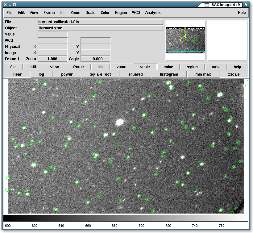
2010-01-05

Fitting of Straight Line

One from most trivial problems of statistical regression analysis is fitting of a straight line. I selected this well-known problem to illustrate
All required code can be found in the archive. Please read README for detailed description of included files.

Reference Data and Solution

As data for a working example, I selected a tabulated values for a straight line from excellent mathematical handbook: Survey of Applicable Mathematics by K. Rektorys et al. (ISBN 0-7923-0681-3, Kluwer Academic Publishers, 1994). The data set is included in the archive as line.dat.

Normal equations:
 14*a +  125*b = 170
125*a + 1309*b = 1148.78
and LS solution:
a   = 29.223
b = -1.913
S0 = 82.6997
rms = 2.625
sa = 1.827
sb = 0.189


Using Minpack

Simple usage of Minpack in LS case is straightforward. One calls hybrd (Jacobian is approximated by numerical differences) or hybrj (must specify second derivatives) and one pass a subroutine to compute vector of residuals in a Minpack required point. Minpack uses Powell's method which combines location of minimum with conjugate gradient method (locate minimum in direction of most steeper slope) far from minimum and Newton's method (fit the function with multidimensional paraboloid and locate minimum by intersection of tangent plane with coordinate axis) near of minimum.

For the straight line, we define

a + b * xi

and minimizing of sum for i = 1 to N:

S = ∑ (a + b * xi - yi

The vector for Minpack is

∂S/∂a = ∑ (a + b * xi - yi)
∂S/∂b = ∑ (a + b * xi - yi)*xi.

The Jacobian is than
∂²S/∂a²    ∂²S/∂a∂b
∂²S/∂b∂a ∂²S/∂b²
or
N          ∑ xi
∑ xi ∑ xi²
All the sums can be found in minfunj in straightlinej.f90.

The call of hybrj search for a minimum of the function. On output, the located minimum is included in fvec and I added a code to compute covariance matrix to estimate statistical deviations of parameters and their correlation.

With gfortran I get the solution on 64bit machine:

....
minfun: par =   29.22344    -1.91302  sum =  82.68976
minfun: par = 29.22344 -1.91302 sum = 82.68976
hybrj finished with code 1
Exit for:
algorithm estimates that the relative error between x and the solution is at most tol.
qr factorized jacobian in minimum:
q:

0.10769513068469699 0.99418396628934158
-0.99418396628934158 0.10769513068469688

r:
152.97596122677001 1371.8039727109779
1371.8039727109779 17.656368881644468

inverse of r (cov):

0.25799238244686612 -2.87651125847342495E-002
-2.87651125847342495E-002 3.20772561895261684E-003

covariance:

1.7777772679919355 -0.19821501231688973
-0.19821501231688973 2.21038374592466315E-002

No. of data = 14
solution = 29.223435764531654 -1.9130248056275454
with dev = 1.3333331421636287 0.14867359368511487
residual sum = 82.689756238430220
rms = 2.6250358130641160
The results must correspond (within precision of tree digits) to the reference solution. As we can see, there is a great discrepancy in deviations of parameters. The Minpack's estimation is little bit optimistic. I think that is due to difference between matrix inversion (which is usually used) and Minpack's covariance estimation. On the other side, the values are the same from practical point of view.

Just for information. The inverse matrix (all by Octave) of Jacobian in minimum is (inv(.))
 0.4846353  -0.0462792
-0.0462792 0.0051833
and the QR factorization ([q,r,.]=qr(.)):
q =
-0.995472 0.095060
-0.095060 -0.995472

r =
-2.0541e+00 -1.2576e+02
0.0000e+00 -1.3150e+03
The Q matrix columns are base vectors (eigenvectors) of solution (the principal axes of covariance ellipsoid) and the diagonal elements are estimates of eigenvalues values (major and minor semiaxes of the ellipse) [l,v]=eig(.).

l =
-0.995457 0.095208
0.095208 0.995457

v =
2.0447e+00 0.0000e+00
0.0000e+00 1.3210e+03

The second supplied routine straightline.f90 does the same work but without explicit knowledge of the second derivatives. The Jacobian is estimated by numerical differences.

The solution can be also done via lmdef, lmder routines in Minpack. It is equivalent to presented solution but doesn't offers generalization toward robust methods.

Robust Fitting

The reference robust fitting procedure is included in rstraightline.f90.

The fitting is logically divided onto two parts. The first part implements minimizing of sum of absolute deviations to get robust estimation of proper solution and MAD (mean of absolute deviations). There is little change with respect on LS because minimizing function have no derivation in minimum. We need another method without using of derivatives. I'm using code prepared by John Burkardt, namely using Nelder-Mead Minimization Algorithm (simplex method). I slightly rearranged the code to nelmin.f90.

The resultant parameters are used to obtain MAD by looking for its median by a quick way algorithm described in Niklaus Wirth's Algorithms + Data Structures = Programs.

The solution is than passed as start point for hybrd which is the second part. The minfun is similar to non-robust version. Only difference between predicted and computed solution (residual) is not directly used, but a cut-off function is used (Tukey's function). This small change does robust fitting itself.
.....
medfun: par= 30.57930 -1.918842 sum= 29.9467137
medfun: par= 30.57930 -1.920842 sum= 29.9506577
ifault= 0 29.940157123526994
t= 30.579306941153348 -1.9198428764730142
4.3939266204833984 2.9615066
minfun: par = 30.57931 -1.91984 sum = 106.17691
.....

minfun: par = 29.24548 -1.91425 sum = 82.69177
hybrd finished with code: 1
Exit for:
algorithm estimates that the relative error between x and the solution is at most tol.
qr factorized jacobian in minimum:
q:

-0.10942034931424138 -0.99399556696996860
0.99399556696996860 -0.10942034931424133

r:

29.315789045435952 295.17538616058539
295.17538616058539 4.3667770003656630

inverse:

5.3177769129754946 -0.52802747846866527
-0.52802747846866527 5.24418460845494372E-002

covariance:

2.7756865626932967 -0.27561118127052436
-0.27561118127052436 2.73727405045027551E-002

No. of data = 14
solution = 29.245477844988198 -1.9142493591979692
with dev = 1.6660391840209812 0.16544709276533920
residual sum = 82.691772460937500
rms = 2.6250678159642766
The output values are practically the same as in non-robust case. Only the difference is estimation of parameter's deviation. I'm using the formula recommended by Hubber (1980), eq. (6.6) p. 173.

The real power of the robust fitting can be easy demonstrated by adding any outlier (point with really different value) to the set, for example, a point with coordinate 10,100. Try to see the robust algorithm in action. It should be practically the same while non-robust solution gives some strange values.

Minpack Fortran Interface

The original Minpack is written in Fortran 77. I'm using modern Fortran (Fortran 90, 95 or 2003) which supports better type checking via interfaces. I prepared such interface which is included in Archive as minpack.f90 and must be passed to compiler during compilation. The module did not changed original API to Minpack routines to prevent any programming errors. So you also must pass to the routines "working arrays" (wa). One is used in modern Fortran more elegant way as automatic arrays (arrays allocated automatically when subroutine is entered and deallocatedon its exit).

Estimation of an initial solution

The solution will not depend on starting point only in linear case. Every complex real) case will lead to non-linear solution with a lot of local minimums which will attract the simplex or the gradient (Powell's method) to a "wrong" solution. To locate global minimum (eg. required solution), I recommends use of genetic algorithms as predictors of a global minimum. The genetic algorithms will locate right minimum with a low precision and we can use some modification of above codes to determine the minimum with required precision.