Improvements in FITSPNG.

With two appendixes.

Fitspng has been originally developed as an utility for a fast conversion of FITS images to PNG format. It is required for our Monteboo data archive for observed image display in an usual internet browser. The conversion can be also required for example for color imaging (look forward).

Some time ago, I did the conversion by two steps: to8bit utility converted normal (16-bit) FITS to 8-bit with an intensity scaling and convert (utility by Imagemagick) done FITS to PNG conversion. The way have been simple for me (I didn't have learn of libpng API) but one is slow due to high system load and storing of middle product on hard disk.

A long time (two years at least), the functionality satisfies of me, but now I have new ideas and I extended functionality of fitspng with respect on rawtran utility and some new knowledge.


Color images

If a multi-color FITS or tree normal (gray) FITSes is passed to fitspng as file to convert than 8-bit color png is created by the algorithm:

1. Fits is opened and recognized as multi-color FITS. All color bands are loaded.
2. The median and mean deviation of positive differences is computed on 10x10 grid (to speed-up the estimation) for every color band. The computation is abandoned when user specified the -fl switch.
3. These estimated parameters are merged with an user specification by -fr switch. Also white balance is setup via CBALANCE FITS keywords of every band or by -w switch.
4. Than every pixel is scaled by specified intensity profile, supplied parameters and white balance.
5. The file is saved as color PNG with RGB colors (without alpha channel). (May be useful add the alpha to image?)

There are two important requirements for the colorization. A simple way how to convert images from a digital camera processed to FITS by rawtran will be:

bash$ rawtran -t 2 IMG_666.CR2 > color.fits
bash$ fitspng color.fits > color.png

Of course, the direct way by ufraw or dcraw will be faster, but you can't apply some enhancing on images and mouse clicking may be really time consuming.

The most important application is on color composing of image data of CCD. The composition itself for tree images in R,V,B filters can be simple:

bash$ fitspng m1_R.fits,m1_V.fits,m1_B.fits > m1_color.png

The default setup of parameters will produce relative nice images but for more nicer images will be need some fine grained tuning via -fX, -w and by specifying of one from transformation functions: asinh, log (magnitude), error function, sqrt and linear transformation. The setup of various parameters by -fX is usually required when a histogram has and non-usual profile (always for non-stellar images).

If you requires nice publishable images, it is absolutely necessary to done basic processing like, dark and flat field correction and detailed photometric analysis. Ideal way is looking for A0 type (not saturated) star and balancing of the images by hand or by -w.

Note, that all single images has its own header with defined keywords which can/are be different. If any keyword is duplicated we get only the first match.

The multi-color FITS has structure:

FITS
+-----------------------------------+
| Primary array - dummy |
+-----------------------------------+
| Extended array - R image |
+-----------------------------------+
| Extended array - G image |
+-----------------------------------+
| Extended array - B image |
+-----------------------------------+


Intensity (flux) scaling

Inspired by Christian Buil, I had implemented asinh intensity profiles together with logarithmic, square root, error function and reimplemented the linear profile. Results are really nice. The profiles are presented on images. BTW, the intuitive color conversion curves which I used with ufraw are similar.

The conversion can be described as an function between output and input data. The input intensity I can be integer or real number without specified range. The output O level has integer range 0 .. 255. The I is transformed to O by

O = f0*f(x) + z0

where f0 is a scaling constant and z0 is black level. The function f(x) can be one from list:

asinh(x)
log(x)
erf(x)
sqrt(x)
x (f0 = 1)

The argument x is computed by a linear transformation

x = (I - t)/s

where t is a "mean" level and s is "mean" deviation. Values t are estimated by fitspng by median of grid pixels with separation of ten pixels (med). The s is determined by the same way on the same set but from positive deviations of t (not from absolute deviations as usually) (mad). Both parameters are corrected by constants u,v:

t = med - 3*mad
s = mad/15

The specified intensity transformation is a product of black magic on images and it can't be derived from an exact axioms. It empirically describes usual parameters of histograms of astronomical images.

The asinh magnitudes are used as photometric product of the Sloan sky survey. They recommends of use of the magnitudes in Lupton et al.(1999) and for color imaging in Lupton et al.(2004).


Working with full directory of images

Fitspng is ideal utility to done fully automatic conversion of fits images. It can be useful for fast look analysis in anyimage viewer or simple file browser. The thumbnails can be generated by command:

bash$ for A in *.fits; do fitspng -a -s 5 $A > ${A%fits}png; done

The switch -s resize the image 5 times.


How to create an animation

If we have images in png format, it is trivial to create an animated gif (with 50 milliseconds delay between images) via convert command of Imagemagic:

bash$ convert -delay 50 *.png animated_sky.gif

Larger animations is preferred to save to mpeg format. It can be created with small script:

---
#!/bin/bash

I=0
for A in *.png; do
for B in $(seq 1 25); do
I=$((I + 1))
N=$(printf "img%04d.png" $I)
ln -s $A $N
done
done
ffmpeg -f image2 -i img%04d.png animated_sky.mpg
---


The ffmepg requires 25 frames per second (at least 10 fps) so we create 25 times links on a single frame. The conversion requires relative small images with approximate size of a post stamp (about 800x600).


Notes.

I spend some time with optimizing of fitspng for speed because the conversion of normal size image gets a few seconds. Unfortunately, any hooks in main cycle are insignificant and, perhaps, the all actions consuming approximately the same part of execution time. The conclusion is that any (great) numerical operations has negligible fluency on execution duration. It is possible to visually inspect of the duration with setup of -v (verbose) switch.

I'm little bit confused about use of keywords of FITS files. They can be defined arbitrary and fitspng can produce fake outputs. I think that the most important is CBALANCE. Fortunately, the keyword can be replaced by -w switch. All others will only put wrong of description of image included in PNG file. The used keywords are listed in source fitspng.c.

The utility is coded in standard C but the coding style is old Fortran like without extensive usage of some user defined types and complicated structure of functions. I believe that the style is fine for coding and long time maintained of filter type utilities. I will not lost in function tree.

I'm expecting additional changes in future.


Examples of images

First image is composed exposition of field of NGC 7635 (Bubble nebula in Cas) acquired during summer 2006 by me and Exebece on MonteBoo Observatory (0.6m refl.) and HaP MK Brno (0.4m refl.) by non-enhanced cameras ST-8 and ST-7 in R filter. The image has been created by composition of 1084 images of total exposure time 95540(!) seconds. The images has intensity scaled by asinh and linear profiles. The differences are most remarkable at central part. The central star is saturated on linear scale, while faint details are visible.

Bubble nebula NGC 7635. Linear intensity profile.

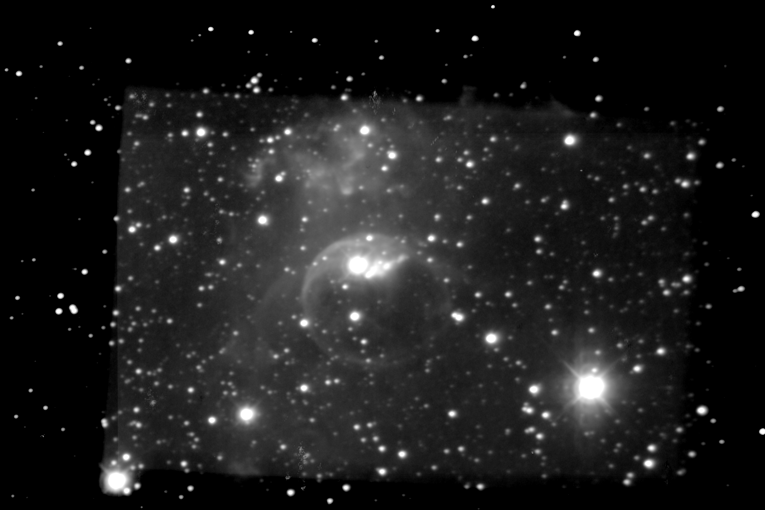
Bubble nebula NGC 7635. Asinh intensity profile.

Second example shows Dumbell nebula (M27) exposed on MonteBoo (0.6m refl.) by Janapka two months ago. It is composition of 3x11 exposures (3x440 sec) in R,V,B filters by our enhanced ST-8 camera. The images has not flat-field corrected.

Dumbell nebula M27. Linear intensity profile.

Dumbell nebula M27. Asinh intensity profile.

So, I strongly recommends use of asinh intensity profiles.

Post scriptum. Scaling to preserve all colors

Dumbell nebula M27. Asinh intensity profile.
Scaled by intensity. Note better preserving of colors.

The paper Lupton et al.(2004) recommends as an optimal way to scale of output image by intensity rather than every single color. You can use the -f switch to invoke it. The key difference with respect to single color scaling is coloring of the saturated objects. The intensity scale algorithm preserves color ratio in (output) saturated regions. The saturated stars have approximate colors opposite with the white color of previous algorithm. Of course, really (on CCD chip) saturated stars are white again. Unfortunately, the saturated stars can create a strange color defect. To remove it, use another black magic.

Post scriptum. I forget attach a graph of all profiles. Please look on the linear (red) and the logarithmic (blue) and asinh (light green) profiles which ideally "interpolates" beween its.
SVG version.



Download of FITSPNG.

Improvements of RAWTRAN

While work on processing of set of images of Venus setting (I will it show soon), I found important bugs and revealed some possible improvements in rawtran utility. Moreover, I also found that only the type zero (default) conversion has worked correctly for all versions up to today. The default choice have composed four RGGB pixels of the Bayer color mosaic to one big grayscale pixel by use of unique weights for separate colors.

The Bayer mosaic is defined as red, blue and two green pixels arranged to rectangular matrix. It means that the number of different colors is tree but we have four pixels on detector matrix. Two green pixels are reserved for single color. Now, we have two choices for output intensities: sum of the pixels or their arithmetical mean. The sum gives precise value in integer numbers but one is two times greater than value of other colors. Opposite with this, the mean gives values of the same order as the red and blue pixels unfortunately with a rounding error as result of conversion between real and integer numbers. I think, the use of the mean and real numbers in FITS should be considered as a smooth alternative when a lot of disk space is available. Also sum of two greens and double values of red and blue can be a nice alternative for 12bit and 14bit A/D converters while we are storing data in 16bit FITSes. The arithmetical mean is the most simple alternative with small lost of precision. Please leave a comment about a preferred way to solve the controversial point.


Color weights

As the first noticeable change, I mention about the color balance (weights) used for conversion of a color based to a greyscale image. Generally, the conversion is done by the formula

I = w_R*R + w_G*G + w_B*B

where I is grayscale intensity, R,G,B are proper intensities in appropriate filters and w_i are a suitable weights. The choice of w_i depends on problem to solve. The setup of w_i is supplied by your camera according to spectral profiles of color device elements and to light conditions of an acquired scene. The photographers perhaps uses the term "white color balance" for the procedure, because it can be easy established by balancing of the coefficients on a white. Now, the camera setup is default. The previous versions used w_i = 1 without possibility to specify by hand. Note that both setups are useful in different situations. The camera supplied setup is ideal for images represents intensities close to reality. The 1's weighting can be useful for detailed spectral examination of images.

The color weights are derived from camera supplied data in field "Camera multipliers". The four numbers B1 B2 R1 R2 are used to estimate of color balance as:

w_R = R1/R2,
w_G = 1,
w_B = B1/B2.

The green band is supposed as basic unit and both remain are relatively scaled. The numerical values agrees with ufraw data. I don't know why also provided "Daylight multipliers" are not used for the reason.

For type zero the image is grayscale and the value is indicated by keyword FILTER which is set to GRAY. Weight factors are not directly included in keywords.


Multi-color fits

The most important change in the code is connected to multi-color (band) fits images. Previous versions has been badly decoding of Bayer's mask (the colors has been swapped). I corrected the bug and changed structure of resultant FITS files.

The effect of correct separation of colors can be easy showed on the image of the spectrum of a white source (data projector) observed through a rainbow glasses (famous paper - diffraction foil glasses). Look on included image for details. I'd correctly decoded the structure of image color mask on the image.

Color image and separated color bands.

Since recent issue, the multi-color FITS has following structure: the dummy primary image array (the header without any data) and tree color (band) extended images. Every header of the extended data contains a new keywords FILTER indicating one from set RED, GREEN, BLUE and appropriate color weight factor included as CBALANCE. Other new keyword EXTNAME is the same as FILTER and can be directly used to select the filter. For example, with ds9 you can directly select blue band by the command:

bash$ ds9 x.fits[BLUE]

The same selection can be done also as x.fits[3]. The file names uses the extended file name syntax introduced by cfitsio library.

Note, about multi-color (band) FITSes. The packaging of more images to one file is frequently used in space astronomy, where an experiment on a spacecraft records a radiation on many different wavelengths. The color mode is particular case of the gadget. The idea can be also extended for including of correction or calibration images or data.

Grid mode

The grid mode (type 1) simply arrange of pixels without collecting or space separating of pixels. I have no idea about any usefulness of the mode. Also I don't fully understand why noise (dark) level and white (saturated) regions are correctly displayed but the mid-level intensities produces grid structure.

8,16,32,-32 bits per pixel images

The output FITSes can have specified bitpix parameter (see man page). It can be very useful when you wanna save fine precision of intensities. The non-integer values are common product of white balancing when type zero conversion is selected. Also, the problem extensive discussed above is suppressed.

I suppose that the mode 16-bit is perfect for storing of raw data, the mode -32-bit for further processing and modes 8 and 32 are unusable. Images with 8-bit depth will usually white due to overflow of image's values over 255. The 32-bit mode only grows range of integer numbers and practically only occupied twice more disk space without any growing of stored information.


Examples of conversion

Basic run (equivalent commands):

bash$ rawtran IMG_666.CR2 > IMG_666.fits
bash$ rawtran -o IMG_666.fits IMG_666.CR2

The produced image IMG_666.fits contains grayscale image with half image dimensions of the original. Please, respect rule: first options than an image to convert.

Process all images in directory:

bash$ for A in *.CR2; do rawtran ${A} > ${A%CR2}fits; done

Process all images listed in a file l.lst:

bash$ for A in $(cat l.lst); do rawtran ${A} > ${A%CR2}fits; done

The file l.lst is usually created by command: bash$ ls > l.lst

Produce of multi-color image and show its green channel (band) in ds9:

bash$ rawtran -t 2 IMG_666.CR2 > IMG_666.fits
bash$ ds9 IMG_666.fits[GREEN]

Produce user's white-balanced multi-color image:

bash$ rawtran -t 2 -w 2.0,1.0,1.5 IMG_666.CR2 > IMG_666.fits

Separate blue color (band) from an image:

bash$ rawtran -t 3 -c B IMG_666.CR2 > IMG_666.fits

The output file roughly corresponds to a filtered CCD image with blue band.


Notes

Please, read source code of rawtran.c to get more detailed understanding of my ideas. I know that code is wrongly structured, it uses of poor data structures etc. but it isn't important for me. Valgrind shows defect free code.

I'm little bit confused about handling with output file. The default setup writes data on standard output which can be strangle for unexperinced users. The suffix swaping is not too elegant for C coding (shell replaces strings more effectively) and unique output filename like rawtran.png is confusing too.

All developing is proceed on images produced by Canon 30D. Be careful when your are working with another digital camera.

Download of RAWTRAN.
An older post about RAWTRAN.

Mandriva's repository of Munipack

Petoš is maintaing himself a repository with some useful software for Mandriva 2009.0. A presence of the current version of Munipack including dependencies (mostly cfitsio) is good news for us. The repository is easy available. Use the command

urpmi.addmedia "Petos" http://physics.muni.cz/~petos/mandriva/2009.0/i586 with media_info/hdlist.cz

to add it to your sources. The repository is for 32-bit branch (i586) . Packages doesn't contains any description and a digital sign. Ones are required to be used together as whole repository (not as independent entities).

BIG THX!

Note. The distribution of binary packages is generally a good idea. But the horrible fragmentation of unix world make me impossible to maintain (at least) some great Linux distribution (Debian, RedHat/Fedora, Mandriva, SuSE, Gentoo,..), *BSD (Free*, Net*, Open*) or Solaris. In despite of the worry, I speculate about this way.

Hády

Hády is a lime-pit on Brno's border. The view to the town center show many millions of lights.

(Canon EOS 30D, 10sec, fish-eye)

These lights strongly illuminates the lime-pit itself. The illumination can be nicely observed on the tree.

(Canon EOS 30D, 16 sec, fish-eye)

The Hády transmitter looks likewise a rocket. Inspect the picture for faintest stars. Our naked eyes revealed only stars up to magnitude two.

(Canon EOS 30D, 32 sec, fish-eye)

Thx for nice accompany to Maceška.

Strange ls & fork

This weekend, I rewrote internal parts of some (darkbat, flatbat, autoflat, meandark, kombine) utilities. The utilities are internally divided into two parts. A wrapper part made interaction of a second part (core of execution) with its environment and user. The core itself provides a required functionality. The wrapper runs the core as a sub-process and both parts communicates via a pipes (output of wrapper is connected to input of core) I did it by a module coded myself (primary for Nightview). The code uses system call fork (along with related ones). Now, It has been replaced by popen system call to simplify and standardize of wrapper's code. The change include some lost of efficiency of code (a shell is invoked) but additional occupied resources are insignificant.

My code to run sub-process work correctly but it has some in-advantages:

• the code is non-standard (developers usually abuse on ones)
• it's complicated to use (requires to use of more complex code)
  

The most important reported error appears for environments with system PATH variable set-up without current directory (without dot). The system reports (Thx to Kočka, M.Zaťko) following strange error:


$ ls * | mdark @
MEANDARK Version 0.1, Copyright (C) 1997-06 F.Hroch, Masaryk
University,Brno,CZ

Subprocess execution failed: No such file or directory: mdark.bin


Nevertheless, both mdark and mdark.bin has correct permissions and the same parent directory. To solve the problem, simply add dot to your system path (for bash: export PATH=$PATH:.) or install any newer version of Munipack.

The separation of code to the wrapper and the core has mostly historical reason. Fortran didn't supported UNIX environment up to version Fortran 2003. All implementations contains some unofficial extensions but it may be syntactically different (for example ifc, g95, gfortran,g77 vs. SUN's Fortran). The separation also provide another additional advantages. The core can be used separately as a part of another great code without any connection to a command line fronted (represented by the wrapper). For example, the core can be easily used in some graphical or web environment.

Also, I found some confusing behaviour of system command ls (list of files in directory). When ls is aliased in zsh (bash?, tcsh?) by the way

ls='ls -F --color'

(color is crucial) we get this really strangle error reporting


$ ls -F --color image.fits | mdark @
MEANDARK Version 0.2, Copyright (C) 1997-08 F.Hroch, Masaryk University,Brno,CZ

image.fits:
The following error(s) has been occured:
input file URL is missing closing bracket ']'
could not parse the input filename: (ffopen)

Of course, it is due to hidden escape sequences which doing output list coloured. I have no idea how to suppress it or how recognize these color marks on input. You has been warned.

On principal pitfall of a star's magnitude calibration

A calibration of magnitudes of an instrumental system to a standard system by an aperture photometry method should be revealing of some unexpected behaviour. Very bright stars are calibrated successfully (also the widely-known method of measuring of an extinction – Bouguer line – gives good results), but fainter (and faintest) stars are exhibiting of some horrible scattering, eg. they're not usable for the calibration. I think, it's result of any inaccurate determination of a sky background. Although our methods for the sky determination are more advanced. The inaccuracy comes from an unstable character of the problem of the aperture photometry.

To show, how some tiny inaccuracy in the background determination fluences to a resultant flux, we will suppose that stars are represented by Gaussian profile

G = G0*exp(-r**2).

An integration in polar coordinates (Jacobian!) of the profile gives us a total flux

F = F0*[1 - exp(-r**2)]

The flux F is equivalent to quantity coming from the aperture photometry, eg. the method which we're uses to estimate of the instrumental magnitude. The real situation is different. We need to subtract the background before summing (integration) of the detected signal on our CCD matrix. The model of detected signal may easy described by

I = G0*exp(-r**2) + B

where B is a constant added to every pixel. It's due to an illumination of the chip by a night sky or any another source. To get aperture photometry, we need subtract of B. That means, that we need to estimate of B by a statistical method with some uncertainty b (b << B).

Let's look to details of determination of total flux with a small error of B estimation. We have a function

I = G0*exp(-r**2) + (B + b)

and subtraction of B leads to

I' = G0*exp(-r**2) + b

so the total measurable flux F' (directly measurable by the aperture photometry) will be

F' = F0*[1 - exp(-r**2)] + π*b*r**2.

This is key moment. Our pitfall is presence of a second term. The first term is total flux of the source and its value is finite and physically limited at any radii. Note that choice of the analytic description of the term is not important. We only requires of integrable function, eg. its integral isn't infinite. Integrable functions has also an appropriate physical meaning. The size of second term depends on uncertainty of estimate of B and on its aperture's area. Because first term is limited, there is a radius where second term dominates over first. The radius depends on the inaccuracy of estimation of B and on object's brightness.

The important characteristics of the measured total flux is its instability. An instability in usual sense means strong dependence of results on input parameters. That is our case. Any tiny (small) perturbation of B lead to strong deviation of output from profile. And, what is more worse, any non-zero value of b (eg. all possible measurable cases) has no limit and the results diverge in in any possible cases (limit of F' is the infinity for the b non-zero)! We won't win!

The findings may interpret results of real measurements. Fluxes of bright stars are (in small apertures) not affected by second term. Faint stars may be too faint and the second term may by more important than the first one at small radii.

Theoretical disturbed profiles

To test the hypothesis, I prepared some graphs. The first one shows of the flux F' of an artificial Gaussian profile disturbed by values of background in range -0.1 to 0.1 (±10%). Both axes takes relative units. The graph is a nice demonstration of drastic fluency of any background estimation error on its resultant profile. Two most important characteristics of error of background estimation are:

• any non-zero value induce significant change of shape of profile
• profile has no limit in infinity

Leo I annotated

Leo I with removed stars

My second graph represents more real situation. There are disturbed fitted profiles of stars on the image of Leo I. The most important change to previous one are:

• magnitude scale
• the profile is non-Gaussian

Set of disturbed profiles of stars on Leo I

The vertical scale shows differences in magnitudes with respect to first aperture. The profile is modelled by a complex function as composition of wighted sum of Gaussian, Moffat and exponential function (see Stetson (1990)). The reliability of the fit can be demonstrated by another image on which the stars has been removed on base of the profile.

Profile of a bright star #1

Final pair of images shows an application of the disturbed mean profiles for two stars. The bright star has no warped profile. Any uncertainty in the sky estimation is insignificant to the total measurable flux of the star. The star is designed by #1 in the above image. The profile shows systematic differences in small radii. It is perhaps due to saturation of the star (the maximum of peak is greater than photon capacity of our CCD detector).

Profile of a faint star #2

The graph for faint star #2 clearly exhibits the effect of the error in estimation of the sky. The profile can be satisfactory modeled if we subtract 0.05 ADU (b = -0.05) from the sky background (determined by Munipack's). We can see, that the precision of the determination of the sky is really important for relative faint stars with its peak only about six thousands and the sky value about six hundredth (ten percent only!). A last point at radius 28 is affected by a hot pixel. The really interesting effects is the deviation of measured values and the modeled profile. The deviation shows some scattering in order of hundredth of magnitude (which corresponds to the precision given by photon statistics). But more important is relative difference between bright and faint star. We can see that the difference depends on aperture which has been used for estimation of magnitude of stars. That means that any magnitude calibration to standard system will depend on magnitude of the star. That is really poor property of the aperture photometry.

Note, that I selected the stars very carefully, because profiles of faint stars are strongly affected by various kinds of defects.

Another point of view offers photon statistics. The middle bright star on the CCD chip gives typically 10^5 photons, so the statistical uncertainty due to only Poisson noise gives about 0.003 magnitude which is about ten factor better than is usually measured.

The key thing of the post (strong fluency of background on aperture magnitudes) is included in paper of Howell (1989). There is only extension some theoretical ideas and another practical test.

Munipack stable release

Yesterday, I finished work on a simple script to make of a regular release of Munipack. Geeks from Fedora Astronomy group included Munipack in their release. Unfortunately, they used a really historical version (it may come from past century). I think, it is due of may unconventional designing and releasing of Munipack (also Nightview) versions. New versions are generated once per day from cvs repository as nightly builds. Many of peoples are supposed that it is a development version only and it isn't suitable as a production release. It isn't true, but all peoples suppose it due to the naming scheme.

To suppress any confusion, the version issue is improved to a conventional naming scheme from now. The "stable" release will be also generated from cvs repository. The generation will less frequent (only once per month), the archive will named as munipack-0.4.?.tar.gz with incrementing only last digit. Also, the archive will generated if the following rules will be satisfied:

• the last changelog record is older then approximately 35 days
• the changelog records are different

I think, it will prevent incrementing of minor version without change of content and it will give me some time for developing and bug-fixing of a new code (you can still use of nightly builds in meantime).

Astronomical image processing guide (How to list of info keywords?)

A great advantage of the FITS format is support of any arbitrary information included into an image file. A place for the info is reserved in header of the FITS file. Every FITS header must contain a set of records (lines) containing certain mandatory keywords. The set may be followed by records with any other keywords.

The mandatory keywords are: SIMPLE, EXTEND and END. All others are optional. The records of header has the fixed structure:

1-8 - keyword
9 - = equal's sign
10-x - value (various lengths)
x -80 - comment (every text following slash '/')

All records are 80-bytes long and there is no separator between ones. The special keywords COMMENT and HISTORY has no defined a structure and introduce any text string (continuation lines are not allowed). Recent recommendations to contents of the records adds physical units to numerical values as a part of comment. Any set of keywords is not widely used. It means that various utilities may used different keyword for the same entity.

The most common keywords are included in following (artificial) example:

SIMPLE = T / file does conform to FITS standard
BITPIX = 16 / number of bits per data pixel
NAXIS = 2 / number of data axes
NAXIS1 = 382 / length of data axis 1
NAXIS2 = 255 / length of data axis 2
EXTEND = T / FITS dataset may contain extensions
EXPTIME = 60.000 / [s] Exposure time
DATE-OBS= '2008-06-06T01:02:41.390' / UTC of exposure start
FILTER = 'R ' / filter
OBJECT = 'Star' / Object name
COMMENT This file was written by XXX.
END

We have more ways to handle with FITS header keywords. Practically, we will need to list of all keywords (as a variant of more or less command on unix's shell) or list of value of some specified record. Both situations can be easy coded. We introduce of utility FITSless which will print all keywords (full header) without any switches and a specified value when any keyword will presented, its value will be printed.

The values are usually different kinds (from computer point of view). For example, the observer's name will coded as a string, an exposure time will a real number, the date of start will a specially formatted string. To print the information, we will use only string representation, but in real code it will be better use of appropriate data type. Unfortunately, there is no simple way how to do it in Fortran, C and cFITSIO under recent versions of ones.

program FITSless

implicit none

integer :: status
! status ... FITS status (0=no error)

integer :: j,blocksize

character(len=666) :: name = 'image.fits'
! name .. fill with name of the image to open

character(len=666) :: keyword
! keyword to print the record

character(len=666) :: record
! header's record

character(len=666) :: value, comment
! record's value & comment

integer :: nhead, hpos
! number of records in header and current position

! get first command line parameter
call get_command_argument(1, keyword)

status = 0
call ftopen(25,name,0,blocksize,status)
if( status /= 0 ) stop 'File not found.'

! list specified keyword or full header
if( keyword /= ' ' ) then

write(*,*) 'List of a record specified by your keyword:'
write(*,*) '-------------------------------------------'

call ftgkys(25,keyword,value, comment, status)
! checking status of the operation
if( status == 0 ) then
write(*,*) trim(keyword),' = ',trim(value),' /',trim(comment)
else
write(*,*) 'Keyword "',trim(keyword),'" not found.'
end if

else

write(*,*) 'Full header list:'
write(*,*) '-----------------'

call ftghps(25,nhead,hpos,status)
do j = 1, nhead
call ftgrec(25,j,record,status)
write(*,*) trim(record)
enddo

end if

call ftclos(25,status)

end program FITSless

The code is self-explanatory, I recommend try this following experiments:

• try give as parameter an arbitrary text string or upper/lower case keywords
• process any printed information by some another text tool (sed, grep,..)
• play with listing of a record on given position in the header
• modify code to read an input file name by command-line parameters

A ridge of algorithms

I spend some time with the growth-curve method during last days. Its looks nice, but relative hard to control.

Some side product of the game is comparison of the original Stetson's algorithm for estimate of the arithmetical mean with new ones. To get mean, Stetson have introduced some rejection-type algorithm. I've no more detailed information about it - there is no reference in source code or a paper. Opposite with this, Munipack estimate of the mean by a method on base of minimisation of a general function. It minimises function in shape of the least-square near of minimum and suppress it to zero otherwise by method of the maximum like-hood. The chapter describing of a robust statistical methods in Numerical recipes is an ideal start point to get detailed view to this field. A source code of Munipack uses of those ideas, but it doesn't describe it. The new estimator has been included to Munipack approximately eight years ago.

I compared of the estimators on case of the ridge of magnitude on differences of following apertures. Both three-dimensional graphs shows number of the differences in cells specified by apertures and its value's ranges. The horizontal (x) axis takes magnitude differences, the horizontal (y) axis takes size of aperture and vertical (z) shows the number of values in that bin interval. The top side of the data cube shows projection of the number of values to a plane. Colors of the histogram maps number of points: dark - near zero, light - near maximum (hundred).

Muniphot's ridge

Stetson's ridge

Both images looks similar. Only one difference is a small systematic shift of the ridge to negative region on Stetson's graph. It is about 0.01 in magnitude, so I think, it is not important in real situations. Perhaps. It may means that the new method for the mean estimations works little bit better.

Ridges height strongly depends on aperture. Small values gives perfect estimation against apertures greater that fifteen (in my case) when the the histogram shows no peaks. The characteristics may be important for growth-curve fitting.

As test data for both graph, I used combined image of M67 as in previous post. However, graphs of ridges looks differently (gnuplot's pm3d feature has been used on graphs here). It is due of my mistake during data processing. The previous perfect ridge with strong peaks at large apertures comes from many zero's differences of bad magnitudes of 99.999. Keep smiling.

Astronomical image processing guide (How to save of an image to a FITS file?)

One of most common operation done on FITS files is creation of a new image. The creation process is straightforward. One is required to have an image (result of a mathematical algorithm) with known dimensions and that's all.

The FITS format supports up to seven-dimensional images without any strict limitation of its axis ranges. Practically, we've some limits due to physical properties of present computers. The most important is a size of the output image. The size is determined (approximately) as a product of image dimensions multiplied by number of bytes occupied by one pixel. For two-dimensional image of 100x100 pixels in both axis, represented by real numbers (4-byte, BITPIX=-32), we got size about 40 kilo-bytes. As we know from previous lecture, the images produced by an algorithm are usually saved as real data to preserve its numerical precision.

As example of a test image, I choose Bessel's function of zero kind J₀ which represents light's diffraction on cylindrical aperture. We can observe of square of Bessel's function in an ideal telescope as the image of a star (of course, we use only J₀ for simplicity, a star will looks differently). J₀ is non-standard Fortran function and may be not supported by all compilers (gfortran does it) so one is optional only and you can play with cosine under a strict-standard compiler.


An algorithm to save an image to FITS file is straightforward:

1. create image as an array
2. fill the array by an image
3. initiate a FITS
4. setup image parameters
5. save the data

program FITSsave

implicit none

integer :: status, bitpix, naxis, naxes(2)
! status ... FITS status (0=no error)
! naxis .. number of axes in the image (we set =2)
! naxes .. dimensions of the image (2-element array)

real, dimension(:,:), allocatable :: d
! data matrix

character(len=666) :: name = 'image.fits'
! name .. fill with name of the image to create

! aux
real :: x,y,r
integer :: i,j

! set dimensions of the new image
naxis = 2
naxes = (/ 100,100 /)

! set bipix of the image (try: 8,16,32 and -32)
bitpix = -32

! create a data storage (allocate memory) for the image
allocate(d(naxes(1),naxes(2)))

! fill image with values
do i = 1, naxes(1)
do j = 1, naxes(2)

! rectangular coordinates
! the left bottom pixel has 1,1
x = i
y = j

! distance from origin
r = sqrt(x**2 + y**2)

! set value
d(i,j) = cos(r/5.0)
!d(i,j) = besj0(r/5.0)
! uncomment for J0 (Bessel function of zero kind)
! J0 represents diffraction on cylindrical aperture
end do
end do

! save the data
status = 0
call ftinit(26,name,1,status)
call ftphps(26,bitpix,naxis,naxes,status)
call ftp2de(26,1,naxes(1),naxes(1),naxes(2),d,status)
call ftclos(26,status)

! free allocated memory
deallocate(d)

end program FITSsave

The code can be compiled and run by

host$ gfortran -Wall -o FITSsave FITSsave.f90 -L/usr/local/lib -lcfitsio
host$ ./FITSsave

the output file is named as image.fits and can be viewed by any FITS viewer, for example by ds9:

host$ ds9 image.fits


Notes.

Any handle with numerical operations in many computer languages may be little bit confusing. Fortran strictly distinguish between integer and real numbers. The notation 3/4 (both integers) products result 0 (reminder is forget), but 4/3 gives 1. Opposite with this, the notation 3.0/4.0 gives 0.75 (two significant places).

The function ftinit (the initial function for FITS file) can create only a new file. There is no way how to replace any existing file. This is simply a feature of cfitsio, not a bug. It means that you must remove the older file image.fits before run FITSsave again.

Astronomical image processing guide (How to list of values of a FITS image?)

Every FITS file is representation of an image usually created by an optical device. The image is quantized (sampled) to elementary cells called pixels. An information knows for any pixel are: a pixel coordinate (Cartesian x,y) and its captured optical flux (CCD's flux is a linear function of captured photons).

The pixels which represents an image, are rearranged and a captured flux is digitalised to a matrix. The matrix is saved to a FITS file by a defined algorithm. The pixels coordinates (integers) are arranged in that matrix by the way:

[M,1] [M,2] .. [M,N]
.. ..
[2,1] [2,2] .. [2,N]
[1,1] [1,2] .. [1,N]

The matrix represents an image of width of N pixels and M pixels of height. The origin and orientation is in usual mathematical fashion.

Every pixel is represented by a number. The kind of the number may be an integer and a real (real numbers are with fractional part). Raw images (pure product of a device) are usually represented by integer numbers in interval from 0 to 65535 (2^16) for CCD and from 0 to 4096 (2^12) for a digital camera. A processed images as result of mathematical operations are saved as a real numbers with floating point. (Arithmetical operations may reduce of its precision). The method (complicated on first sight) to store of data reflects many of astronomer's needs and save your disk space. The data representation is coded in parameter BITPIX in the fits header by the way (not all possibilities are included):

BITPIX bytes type range of values
8 1 integer 0 .. 255
16 2 integer 0 .. 65535
32 4 integer 0 .. 4294836225
-32 4 real -1e38 .. 1e38 (7 digits)

An operation on a image included in a FITS file is relative easy. Follow the instruction:

1. open of FITS
2. get of its size (width, height)
3. allocate memory for a matrix
4. read data
5. play with data

Fortran offers a very effective way for manipulation with matrixes. For a matrix D, we can select an i,j-element as D(i,j), a i-row D(i,:),i-column D(:,j) or submatrix D(1:10,50:60).

program FITSlist

implicit none

integer :: status, bitpix, naxis, naxes(2)
! status ... FITS status (0=no error)
! naxis .. number of axes in image (we require =2)
! naxes .. dimension of the image (2-element array)

integer :: i,j,blocksize,pcount,gcount,minvalue
logical :: extend, simple,anyf
! required by cFITSIO

real, dimension(:,:), allocatable :: d
! data matrix

character(len=666) :: name = 'image.fits'
! name .. fill with name of the image to open

status = 0
call ftopen(25,name,0,blocksize,status)
call ftghpr(25,2,simple,bitpix,naxis,naxes,pcount,gcount,extend,status)
allocate(d(naxes(1),naxes(2)))
call ftg2de(25,1,minvalue,naxes(1),naxes(1),naxes(2),d,anyf,status)
call ftclos(25,status)

! print value of a random pixel
write(*,*) '# d(1,1)=',d(1,1)

! print last tree values of first row
write(*,*) '# d(1,-10:)=',d(1,size(d,2)-3:)

! print of a submatrix with indexes
do i = 1,10
do j = 50,60
write(*,*) i,j,d(i,j)
end do
end do

end program FITSlist

The output of the code can be saved to a file by sequence of commands:

host$ gfortran -Wall -o FITSlist FITSlist.f90 -L/usr/local/lib -lcfitsio
host$ ./FITSlist > pixels

and easy plotted in a gnuplot with the command:

gnuplot> splot 'pixels'

How aureole shades stars

The photometry (magnitudes of stars) produced by Munipack is an aperture photometry, which means that a magnitude is determined only as a sum of a flux inside an artificial aperture. The aperture photometry is sufficient for a relative comparison of stars. It should be very useful in many applications like observing of variable objects (variable stars, asteroids, afterglows,..), but there are many of additional requirements (calibration of photometric system, precise photometry,...) in which the aperture photometry start to fail.

Briefly, an image of a star is theoretically a point, but Earth's atmosphere and telescope's optics spread the point to a blob with Gaussian central part and an outer parts showing an "aureole". The problem of the aperture photometry is our ignorance of outer radii which may include an important fraction of a total flux. If we will ignore the aureole's flux, any magnitudes will depends on atmospheric conditions (seeing spreads stars with dependence on its air mass or a night) and on magnitude of the magnitude (A golden rule of differential photometry is to compare objects with similar magnitude). It means that precise photometry requires more sophisticated approach.

Described problems bothers CCD's photometrics for a long time. They are described in articles of classics at 80'. Howell(1989) points to properties of the aperture photometry for differently bright stars. He shows that total flux of bright stars is determined relative precise, but any small error in determination of background for any faint star strongly affects total fluxes. The solution of the problem did published Stetson(1990) in that great article. He developed a method on base of cumulative distribution of magnitudes of stars (in astronomical dialect the grow-curve method). Please read the paper, I have no time to transcribe it here. The most important ones (from my point of view) are: The grow-curve method is complement to PSF method (PSF <=> precise relative magnitude, grow <=> precise calibrated magnitude). The model of cumulative profile of the star as an integral of PSF can be described by a sum of analytic functions (Gaussian, exponential and Moffat - Moffat is generalisation of Lorentz).

The grow-curve method for a large radii can be described by Moffat's function ~1/(1+r^2)^A (A=2 for Lorentz). We suppose that all stars on the image has the same cumulative (grow-curve) profile (integral of PSF modeled by Moffat). To construct of the mean grow-curve for all stars with no matter to its brightness, Stetson uses ratio of fluxes in et sequentia of apertures, eg. the following differences of aperture's magnitudes.

M 67

I try it on image of the M 67 open stellar cluster exposed on 2008-02-26 at R filter via 0.4m telescope at HaP MK Brno. The standard Munipack run has been done. About 250 stars has been found. The results included in graph in fashion of the Stetson's article are included.



I take out of these basic fact from the graphs:

• The scatter of the points is relative great over five magnitudes (not all are included). It is due to random errors, disturbance of magnitudes of overlap stars, wrong determination of background for faint stars.
• A pretty description of magnitudes displays frequency of magnitudes in an interval of difference magnitude and apertures. There is a spine visualising of most frequent values of the variables. I'd pleasure from behaviour of the spine at large radii where the values converges to zero. It means that the robust mean algorithm used in Munipack to determine of sky level is really good.
• The graph show differences about 0.1 magnitudes at radii usually applied to photometry. The function is not a profile itself. It means that the difference between a real and determined magnitude will a few tenth of magnitude. In other word, the calibration of Munipack's aperture magnitudes will depends on actual observation conditions and the calibrations derived from the magnitudes will contain an systematic error which will be depend on magnitude of a star.

Astronomical image processing guide (How to open a FITS image?)

A structure of a FITS file is a little bit complicated, but not too much. The FITS itself includes a header and a data part. The header of an image consists from meta-information about the image. The most important are the size (width and height) and data representation of the image.

The header is set of 80-byte (character) length records. Every record is represented by text line with structure:
KEYWORD = VALUE
The KEYWORD must be no longer than 8 characters. The '=' must be in 9 column. The width and height of an image is coded by the way:
NAXIS1 = 1628
NAXIS2 = 1236

How to get an image size?

To get this basic information by use of the cfitsio library, we can use of the piece of the code (source code):

! to compile: gfortran -Wall -o FITSsize o.f90 -L/usr/local/lib -lcfitsio

program FITSsize

implicit none

integer :: status, bitpix, naxis, naxes(2)
! status ... FITS status (0=no error)
! naxis .. number of axes in image (we require =2)
! naxes .. dimension of the image (2-element array)

integer :: blocksize,pcount,gcount
logical :: extend, simple
! required by cFITSIO

character(len=666) :: name = 'image.fits'
! name .. fill with name of the image to open
status = 0
call ftopen(25,name,0,blocksize,status)
call ftghpr(25,2,simple,bitpix,naxis,naxes,pcount,gcount,extend,status)
call ftclos(25,status)

if( status == 0 ) then
write(*,*) 'The image ',trim(name),' has the size:',naxes
else
write(*,*) 'The image "',trim(name),'" not found or not accessible.'
end if

end program FITSsize

The code may by compiled by command:

host$ gfortran -Wall -o FITSsize FITSsize.f90 -L/usr/local/lib -lcfitsio

where switch -Wall prints some warnings, -o specify name of the generated binary file (name of the routine), -L points path to cfitsio library (may be omitted, usually any system directory) and -lcfitsio links cFITSIO library (libcfitsio.a).

Type:

host$ ./FITSsize

to run. The utility will try to open file named as 'image.fits' (can be changed in declaration name = 'image.fits'). If this file is accessible it will print the size of the image. If the name can't be open, an error will appeared.

This code demonstrates basic idioms of FITS-specific ones:

• its look horribly
• there is a lot of declarations which meaning is too hard to remember
• the variable status must be set to zero before calling of any of cFITSIO routines
• the name of the image to open is a second argument to ftopen
• the routine ftghpr reads important parameters (coded by KEYWORDS as above) of the image

Astronomical image processing guide (Intro)

From time to time, I'm thinking about the most useful way to process of an astronomical image data. An use of wide-known software package utilities like Gaia, ds9, IRAF may be better or worse in comparison of a direct coding of a self-made routine? Both approaches has its own advantages and disadvantages so, I think, there is no an universal way to process its. For example, a lot of work can be done inside IRAF's (http://iraf.noao.edu/) environment, but sometimes may be faster and more suitable of coding of an own utility. Both approaches may be possible useful and important especially for a particular processing. Also, I thinks the develop of any own routine may be much, much better and simpler then use of prepared ones. While there is a lot of documents describing of various software packages, the processing in a computer language is described poorly. That's why I'm starting write this guide.

The basic operation to work with data is data file handling. A FITS format (http://heasarc.gsfc.nasa.gov/docs/heasarc/fits.html) is a wide-used format to storing of an astronomical data including both an images and a data tables. A general structure of FITS files may be really very complicated. Fortunately, W. Pence and etc. made the cFITSIO library to provide of a standard way to create, open and modify of any FITS files. The library offers interfaces for C and Fortran languages. There is also a lot of wrappers to others (Perl, Python, C++, ..). I'll use of Fortran (fortran 90/95/2003 dialect) in this guide to create a simple code but the change to C (for example) is straightforward.

A computer library (like cfitsio) is a file with a special structure which includes a set of (useful) functions. The file is usually created by compiling of a computer language (cfitsio is in C) to a machine-specific code.

How to install an environment to open FITS files?

1. Use of your package system and install gfortran (Fortran compiler).
2. Use of your package system and install cfitsio.

ad 1). The gfortran is included in most modern Linuxes. Its is possible to use also Intel's ifort (apparently faster). Solaris offers f90/f95. The GNU g95 provides binaries for other systems (BSD's, Mac OSX, ..).

ad 2) Many modern distributions (Debian, Ubuntu, Fedora..) offers cfitsio as a package. If your doesn't, download directly tarball. Move it to /tmp and execute:
host:/tmp$ tar zxf cfitsio-x.y.z.tar.gz
host:/tmp$ cd cfistio-x.y.z
host:/tmp$ ./configure # check output
host:/tmp$ make # compile
host:/tmp$ su # switch to root account
host:/tmp$ make install # install to /usr/local

To install it in an another place use --prefix parameter for configure (./configure --help). To uninstall it, type (as root) make uninstall. A successful installation is indicated by presence of drvrsmem.h,fitsio.h, fitsio2.h and longnam.h in /usr/local/include and libcfitsio.a in /usr/local/lib.

The Fan on Leo I Revealed

The unidentified fan on bottom edge of the image of Leo I has really simple explanation! Rays are diffraction patterns of Regulus lying twenty arc minutes bellow Leo I. The connection has been revealed by readers of IAN.cz. Thank you very much! It is a very good example how Internet can help expand of a knowledge. I have no explanation how I had ignored this fact. I inspected the position of Leo I with Xephem and I miss the critical proximity and I had in mind that the Leo I falls to the head of Leo. So don't forget look under legs when you are watching of the sky...

When I play with raw images, I inspect ones by an animation. The animation (warning 36M!) shows "a shut of the fan" near of its end so I gather from the investigation that the light pollution is due of a Earth's source. The animation shows a relative motion of the telescope (corrected by pointing), an airplane, cosmic-ray event and inner lights of our dome.


A last step to full explanation of the secret has been done by exebece. It take note that all stars are fainter at the end of the observation run. The instrumental magnitudes of the star UCAC2 36118678 shows rapid fall of its light fluxes. An explanation of the fainting is direct. The aperture of the telescope, controlled by the siderical motion, has been occult by our dome. A creativity of all possible mistakes by me is unbelievable...;)

The Zodiacal Light

A mysterious zodiacal light can be sight at the season of the spring equinox. The weather and the sky prepared for us an absolutely excellent spectacle during last weekend and we was able to view the zodiacal light for the first time!

We made three journeys to Rojetin's airport. At first evening, we did sight some lights above west's horizont, but we did understand that we did sight the zodiacal light after that it disappeared. Also, we made some photos but with ISO 600 only so all images are underexposed and noisily. Our second journey was the most successful. Horrible clouds has dissolved and we sight clearly the zodiacal light with help of our fresh experience. Our last journey started really optimistically because the sky has no clouds for whole day. Unfortunately, an atmospheric front moved to west's horizont and it did scatter a light over the zodiacal light. We did not sight anything.

The first image shows the zodiacal light during our second journey. The zodiacal light is a white difuse part of sky below Pleyades (rightly). A head of Taurus is at center of the image, Orion is on the left. Do you know where a white dwarf can be found? The image was acquired at 2008-03-30, 18:05 UT, EOS 30D, f/2.8 fish-eye, ISO 1600, 32 sec and processed by Ufraw+dcraw (histogram equalisation, wavelet denoising) and Gimp (unsharp, resize). The camera configuration and processing is common to all related images (larger).

Next two images recorded a passage of the ISS and Jules Verne spacecrafts during evening of 2008-03-31, 17:39 UT (the same camera configuration). I prepared two versions of the image in a large format (I believe) useful for wallpapers.

I dedicated, inspired by Paulie, the 31's evening to made a sequence of horizont-centered exposures. Unfortunately, clouds has been brighter than the zodiacal light.

Thx to all peoples of my team: Janis, Petoš, Barča, Ushas, Maceška, Jarda, Janapka, Kočka, Fantom, Ondratik and Paulie.

Color transformation

This record is just for future references.

Some time ago, I got profiles of transmissivity of our new set of photometric UBRVI filters (thx to K.Navrátil). The filters are offered as a part of the official SBIG's accessories. Profiles of trasmissivity of the filter set and Landolt's (Astron. J. 104, 340 (1992)) filter set is displayed on the image:(in PDF). All filter profiles together with various useful files are included in archive newfilters.tar.gz.

A knowledge of the profiles enable us to create a transformation between our and Landolt's filters set. The transformation is constructed only on base of the filter's transmissivity. That means that another one made as a product of a real measurement will perhaps different due to any different spectral sensitivities of others parts of our optical equipment (mainly telescope, detector and atmosphere). We are use the transformation between our set {|u>,|b>,|v>,|r>,|i>} and Landolt's {|U>,|B>,|V>,|R>,|I>} as the matrix equation

|u> = U><U|u> + |B><B|u> + |V> <V|u> + |R><R|u> + |I><I|u>
|b> = U><U|b> + |B><B|b> + |V> <V|b> + |R><R|b> + |I><I|b>
|v> = U><U|v> + |B><B|v> + |V> <V|v> + |R><R|v> + |I><I|v>
|r> = U><U|r> + |B><B|r> + |V> <V|r> + |R><R|r> + |I><I|r>
|i> = U><U|i> + |B><B|i> + |V> <V|i> + |R><R|i> + |I><I|i>

where the matrix elements are defined as area determined by the product of the transmissivity of the filters. For example

<U|u> = ʃ U(λ)u(λ) dλ
<B|u> = ʃ B(λ)u(λ) dλ

...

for all wavelengths λ = 0 to ∞. The results of the integration and solution of the matrix equation are in the table:

0.5051 -0.0131 -0.0008 -0.0001 -0.0000
0.1680 2.5373 0.0233 0.0028 0.0008
-0.0010 0.0587 1.4170 -0.1299 -0.0381
0.0003 -0.0104 -0.0828 0.9252 0.0747
-0.0000 0.0009 0.0073 -0.0460 1.0063

The filter based transformation between our instrumental magnitudes m_i for i = U,B,V,R,I and Landolt's M_i is described by the term

m_u - M_U =
-2.5( log10 <U|u> + log e (<B|u> + <V|u>+<R|u>+<I|u>)/<U|u>)
+ <B|u>/<B|b> (M_B - M_U)
+ <V|u>/<B|b> (M_V - M_U)
+ <R|u>/<B|b> (M_R - M_U)
+ <I|u>/<B|b> (M_I - M_U)
...

(analogically for other filters). The numerical results are:

m_u - m_U = 0.8110 - 0.0260 (m_B - m_U) - 0.0016 (m_V - m_U) - 0.0002 (m_R - m_U)

m_b - m_B = -1.203 + 0.0662 (m_U - m_B) + 0.0092 (m_V - m_B) + 0.0011 (m_R - m_B) + 0.0003 (m_I - m_B)

m_v - m_V = -0.1838 - 0.0007 (m_U - m_V) + 0.0415 (m_B - m_V) - 0.0917 (m_R - m_V) - 0.0269 (m_I - m_V)

m_r - m_R = 0.1338 + 0.0003 (m_U - m_R) -0.0113 (m_B - m_R) - 0.0895 (m_V - m_R) + 0.0807 (m_I - m_R)

m_i - m_I = 0.0870 + 0.0009 (m_B - m_I) + 0.0073 (m_V - m_I) - 0.0457 (m_R - m_I)

Detailed description of the used method and an application to our old
filters can be found in Janis's bachelor work (in Czech).

(The old school typhographics rules! A "modern" graphics technologies doesn't supports a little bit complicated typesetting as (La)TeX did twenty years ago.)

Spectrum from Heavens

Hrošátka (group of my students) experimented with our new SGS spectrograph on last Thursday. It was of our first real contact with the device so any basic operation was hardly for us (arranging, focusing, pointing, exposing). We acquired a few spectra of some bright objects to test of our equipment. I see, we will need a lot of fine tuning and a lot of experiences in observation and data processing to get a day-to-day usable spectral apparatus. Also, I meet again with CCDops utility. It works nicely under Mac OS X, but it is still hardly to use.

All the spectra has been acquired on evening 2008-03-13 by SGS spectrograph in a low-dispersion configuration and mounted on Celestron 14" with ST-8 XME camera as a detector. All images has been processed by the same way as previous ones. The wavelength calibration is only preliminary.

A first object to acquire was the Moon. It is bright and easy to point. Moreover, the spectrum of the Moon is practically identical to the Sun's spectrum. The resultant spectrum shows a great peak of a continuum radiation modulated by some absorptions lines. The great peak practically visualise the spectral sensitivity of our CCD camera. There are only strong lines due to a non-perfect focusing.


As second object, we acquired Sirius. Sirius is a hot star with spectral classification A0. The spectrum shows practically only strong hydrogen lines of the Balmer's series.


A little bit fainter star was Procyon of a spectral class F5. The hydrogen lines are suppressed and only marginal features are visible. I selected this spectrum as an illustration of an image of a spectrum on the CCD chip.


A high pressure sodium streetlamp has been tried as a possible calibration source. The spectrum is quite different due to a non-thermal mechanism of lighting. Unfortunately, the spectrum is included in all other specters as emission lines. The sky's spectrum is also practically identical. Note, that spectra by a Ch. Buil shows some differences.
Thx to my students Maceška, Kočka and Peťoš for a great help. Especially, Maceška bravery controlled of our notebook when she had a broken leg.

Update: Raw images of spectra are available on Petoš's blog.

Leo I

One of twelve known companions of our Galaxy (Milky way) is a dwarf galaxy Leo I. The object is projected to a head of Leo constellation with look like a faint star cluster of an approximately dimension of five arcmins and with its total visual magnitude about ten. Leo I is 250 kpc far from us (Milky way has 30-40 kpc in diameter) so its linear dimension is quarter or half of kiloparsec(!). The estimated number of stars (with sun's mass) is 10⁹ (Milky way contains about 10¹¹ of stars). The galaxies like Leo I appertains to a class of dwarf spheroidal galaxies (dSph).

A relative proximity of this kind of galaxies enables us to study of various details not accessible for remote ones. Especially, it is possible to resolve of individual stars and to measure of its magnitudes and spectra. The measurements gives direct values of a dispersion velocity (The dispersion velocity can be determined by estimation of a width of a spectral line raised as a mean of velocity differences of individual stars. The value is greater for faster stars and doesn't depends on a relative velocity of a galaxy's center of gravity.). Velocity measurements are a tool to mapping of the gravitational potential. If any outer fields are negligible, the potential is formed by a distribution of stars. It is worse that the distribution of stars is formed by potential. Fortunately, the simultaneous fitting of both quantities gives right results. But there is problem with observed discrepancy between number of stars (the projected surface luminosity) at a some radius from a core and the dispersion velocity at the same place. That is widely known problem of "dark matter" because the velocity is greater than we are expecting from observations of number of stars with an usual luminosity.

Only for my interest, I made an observation of Leo I on MonteBoo Observatory. A resultant image has been acquired by composition of a series of images at 2008-03-06 between 19:51 and 22:15 UT (totally 5160 sec) by our 0.6m telescope at R band. The Leo I itself is situated to the center of the image as a faint stellar cluster (compare with image of D. Malin on APOD). A graph by a paper Walker et al.(2007) (it contains recent measurements of the dispersion velocities for seven dSphs) is placed to the image. The original graph is scaled to match of the position and the angular scale of Leo I. The solid line fits the measured velocity dispersions in km/s. The horizontal axis represents a distance from its center in parsec (the range is: 0 to 2kpc). The hashed line is a King's model for the luminosity which roughly corresponds to density of stars in the image. For better description, read the original paper. The discrepancy between the luminosity and the velocity is clearly visible. The velocity is a constant at radius where the density of stars is relative low. Note, that potential (velocity) falls rapidly when no matter is presented.

Moreover, the image exhibits a lot of defects over Leo I itself. "Stairs" at edge of the image together with white corners demonstrates a pointing mode of the telescope during a long time series. The effect is intensified by correcting of the image for its median. The median also suppresses a light pollution due to an unidentified near light source. The pollution creates a fan of rays at bottom of image.

Kotvrdovice's airport

My Sunday's afternoon trip to Moravian Karst finished on Kotvrdovice's airport. The airport is covered by grass plot except a small part of concrete and perhaps it's an airport for sports planes. A horizon is near of ideal but the concrete surface is in proximity of Kotvrdovice (and public lighting) itself. The airport is about two kilometers from Kojál transmiter.

Kotvrdovice's airport facility and runway.

View to Kojál.

Archive of our observations

Four years ago, I wrote a really simple database engine for our observations. The data are indexed one per day and stored in a database (sqlite, more sophisticated engines need a server) and the served via at the most simple web interface. This philosophy satisfy all our needs so there is no reason for a change.

Now, I'm moving our old software to a new computer so I made a small improvement to database by adding of a new Reference column to front (year) page. It provide a possibility to back-linking of some results to the original data.

The data archive has a link in my links.

Eclipse of the Moon

Last week has been dominated by eclipse of the Moon. We had a trip for possible locations (with a romantic ruins on the horizont) week ago. Our weather condition was really poor during eclipse time so the phase of totality has been obscured by cloud completely. There are a few pictures and one animation to illustrate the times.

The trip is also documented on pages of Janapka and on Galaxy tea.

A lake under Apollon's temple at winter. Apollon's temple is a part of Lednicko-Valtický areál.

A detail.

A lake below Apollon's temple. Pálava on horizont.

15cm telescope of HaP MK Brno during eclipse. Thx Peťoš.

A link to animation of clouds and halo before eclipse.

First spectra by SGS

Last year, we purchased the SGS spectrograph. I spend today's afternoon by acquainting myself with the device. First images looks really amazing. All ones has been acquired in my office with a scattered radiation of a fluorescent lamp as a light source with our new ST-8 XME camera as a detector. Compare my findings with its spectrum.

An image of a spectrum of fluorescent lamp in low-resolution mode of SGS. The wavelength interval is about 300 - 900 nm. Ultraviolet is on the left, red is on the right.

An image acquired in high-resolution mode. Wavelengths in interval 490 - 650 nm. The orientation is the same as in previous case. The image covers approximatelly central quarter of the low-resolution spectra (try find of Tb - Eu series between two strong lines).

The image of the same lamp acquired by a digital camera (Canon EOS 30D) and a simple CD spectrograph for comparison. You can simply identify global spectral features. The strong red line corresponds to the strong line on the right on high-res image of spectra. The green line is the strong line on the left of the same image. The lighter horiznotal line has been used for construction of a first graph on image below.

A calibrated graphs of spectra of the images above (click for original size). Top to bottom: spectrum by CD's "grating", low-resolution of SGS, high-resolution of SGS. The graphs exhibits different spectral resolution of all "instruments" (look on series of Tb and Eu at 570-600 nm) and different spectral sensitivity (color graphs, line at 550nm).

Once, the spectra looks really fine, I'v worries about simple use of our equipment. The CCD can be connected to spectrograph only without filter wheel (due to focusing range) but the removing of the wheel is really complicated and delicate operation.

Rojetín - preliminary 21 mag/"

Today, I processed zenith's images of night sky taken during Saturday's trip to Rojetín. Original RAWs has been converted to FITSes by rawtran.

Dark frames has been processed by mdark utility from Munipack. My fast statistical analysis of a noise of the dark images shows pretty Gaussian histogram with center on level 380 and thickness about 7-8. The noise looks little bit greater then noise of our CCD camera at the same temperature (approx. 0°C). The dark frame reveals a smooth electro-luminescence at a corner probably due to a fast transfer of electrons to an A/D converter.

The converted light images has been corrected by the darks. The application claimed a small modification of rawtran because our camera detects a gravity direction and it automatically rotates images to a portrait orientation and rawtran needs rotate it back (if not, the size of lights and darks are different).

A combination of our Canon 30D camera and our 17mm Canon's fish-eye gives us a scale about 21 pix/°, eg. 2.9' per pixel near center of projection. I determined the value by use of two stars (therefore it is preliminary only!). A precise analysis will need construction of a model of the projection.

All light images has been processed by muniphot by a standard way (determination of a mean background, finding of stars and an aperture photometry). To my surprise, it works without any troubles. The number of found stars for 3-σ is almost 13 000 and for 1-σ over 50 thousands (!). The limiting magnitude of stars (1-σ) has been determined approximately on 10 magnitudes for 30sec in wide-band of sensitivity of our camera. The photometrical calibration (determination of a zero level for instrumental magnitudes by using of known stars) shows a relative great scatter for stars in the interval 2-7 mag. The position on the chip (near center or border) along with position in Milky way doesn't matter. Opposite with this, the color of stars is important and red stars are unusable for it. It may be due to a mist (or another reason).

My determination of sky brightness on place non-confused by Milky way but near of zenith gives value of 21.0 magnitude per square arcsecond with uncertainlity not better than 0.5. So the place satisfy of hard requirements for our observations.